
Image Classification - Machine Learning With Cats and Dogs
This tutorial will go over multiple machine learning models that will try to classify images. We will create models that will classify images as having a dog or a cat pictured in them, and analyze the models’ correctness.
Preparing The Model
To begin, we will first import all the neccessary packages.
import os
import tensorflow as tf
from tensorflow.keras import utils, datasets, layers, models
from matplotlib import pyplot as plt
import numpy as np
Next, we will download all the data that we will analyze, namely the photos of cats and dogs.
# location of data
_URL = 'https://storage.googleapis.com/mledu-datasets/cats_and_dogs_filtered.zip'

# download the data and extract it
path_to_zip = utils.get_file('cats_and_dogs.zip', origin=_URL, extract=True)

# construct paths
PATH = os.path.join(os.path.dirname(path_to_zip), 'cats_and_dogs_filtered')

train_dir = os.path.join(PATH, 'train')
validation_dir = os.path.join(PATH, 'validation')

# parameters for datasets
BATCH_SIZE = 32
IMG_SIZE = (160, 160)

# construct train and validation datasets
train_dataset = utils.image_dataset_from_directory(train_dir,
                                                   shuffle=True,
                                                   batch_size=BATCH_SIZE,
                                                   image_size=IMG_SIZE)

validation_dataset = utils.image_dataset_from_directory(validation_dir,
                                                        shuffle=True,
                                                        batch_size=BATCH_SIZE,
                                                        image_size=IMG_SIZE)

# construct the test dataset by taking every 5th observation out of the validation dataset
val_batches = tf.data.experimental.cardinality(validation_dataset)
test_dataset = validation_dataset.take(val_batches // 5)
validation_dataset = validation_dataset.skip(val_batches // 5)
The following code block is helpful by making the reading of data much faster. We will also store the class names of “cats” and “dogs” in a variable.
class_names = train_dataset.class_names
AUTOTUNE = tf.data.AUTOTUNE

train_dataset = train_dataset.prefetch(buffer_size=AUTOTUNE)
validation_dataset = validation_dataset.prefetch(buffer_size=AUTOTUNE)
test_dataset = test_dataset.prefetch(buffer_size=AUTOTUNE)
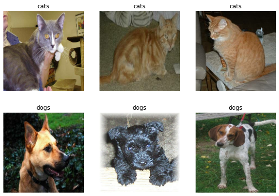
Now, we can fetch a sample of the data. The following function retrieves and shows three cats and three dogs at random.
def random_pets():
  train_dataset.take(1)

  plt.figure(figsize=(10, 7))
  for images, labels in train_dataset.take(1):
    num_cats = 0
    num_dogs = 0
    # cycle through an arbitrary number of images to "guarantee" 3 dogs and cats
    for i in range(20):
      # if it is a cat and we haven't filled the top row yet:
      if(class_names[labels[i]]=="cats" and num_cats<3):
        ax = plt.subplot(2,3,num_cats+1)
        plt.imshow(images[i].numpy().astype("uint8"))
        plt.title(class_names[labels[i]])
        plt.axis("off")
        num_cats += 1

      # if it is a dog and we haven't filled the bottom row yet:
      elif(class_names[labels[i]]=="dogs" and num_dogs<3):
        ax = plt.subplot(2,3,num_dogs+4)
        plt.imshow(images[i].numpy().astype("uint8"))
        plt.title(class_names[labels[i]])
        plt.axis("off")
        num_dogs += 1
Now, let’s see the function work:
random_pets()
Lastly, let’s get some more information on our test data.
labels_iterator= train_dataset.unbatch().map(lambda image, label: label).as_numpy_iterator()

num_dogs = 0
num_cats = 0
for label in labels_iterator:
  if(label == 0):
    num_cats = num_cats + 1
  else:
    num_dogs += 1
print("Number of cats:", num_cats)
print("Number of dogs:", num_dogs)
Number of cats: 1000
Number of dogs: 1000
As we can see, there are equal numbers of photos of dogs and cats. Therefore, our baseline machine learning model would perform at about 50% accuracy.
First Model
The first model we will create involves using Conv2D, MaxPooling2D, Droupout, Flatten, and Dense layers. After manipulating the order of the layers and changing the Dropout rate, the resulting model turned out to be the most efficient.
model1 = models.Sequential([
    layers.Conv2D(32, (3, 3), activation='relu', input_shape=(160,160, 3)),
    layers.MaxPooling2D((2, 2)),
    layers.Conv2D(32, (3, 3), activation='relu'),
    layers.MaxPooling2D((2, 2)),
    layers.Dropout(0.4),
    layers.Flatten(),
    layers.Dense(2) # number of classes
])
Next, we must train our model to see how it performs.
model1.compile(optimizer='adam',
              loss=tf.keras.losses.SparseCategoricalCrossentropy(from_logits=True),
              metrics=['accuracy'])

history = model1.fit(train_dataset,
                     epochs=20,
                     validation_data=validation_dataset)
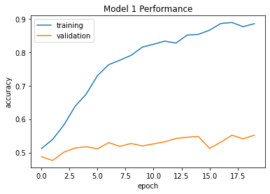
We can see that the validation accuracy stabilized between 55% and 60%. This appears to be just slightly better than our baseline model that would simply take a random guess, with a 50% chance of getting it right. However, we can see that the training accuracy is far higher than the validation accuracy, so we can conclude that our model has been overfitted and that we need to change our model.
plt.plot(history.history["accuracy"], label = "training")
plt.plot(history.history["val_accuracy"], label = "validation")
plt.gca().set(xlabel = "epoch", ylabel = "accuracy", title="Model 1 Performance")
plt.legend()
Second Model
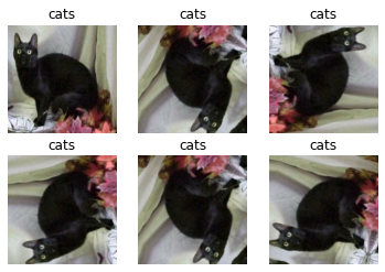
In our second model, we will combat the overfitting issue by creating layers that will provide rotated and fliped versions of the photos. That way, it can tell whether the photo is of a cat or dog despite the orientation of the photo. The first thing we will do is demonstrate the layer that will perform flips, and output sample photos.
flip = layers.RandomFlip()

for images, labels in train_dataset.take(1):
    ax = plt.subplot(2,3,1)
    plt.imshow(images[0].numpy().astype("uint8"))
    plt.title(class_names[labels[0]])
    plt.axis("off")
    for i in range(5):
      ax = plt.subplot(2,3,i+2)
      plt.imshow(flip(images[0]).numpy().astype("uint8"))
      plt.title(class_names[labels[0]])
      plt.axis("off")
    break
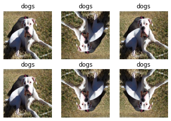
The next thing we will simulate is rotating the photo. We will do the same thing as above, but using a different layer.
# create rotations of th photo in any possible orientation:
rotate = layers.RandomRotation(1)

for images, labels in train_dataset.take(1):
    ax = plt.subplot(2,3,1)
    plt.imshow(images[0].numpy().astype("uint8"))
    plt.title(class_names[labels[0]])
    plt.axis("off")
    for i in range(5):
      ax = plt.subplot(2,3,i+2)
      plt.imshow(rotate(images[0]).numpy().astype("uint8"))
      plt.title(class_names[labels[0]])
      plt.axis("off")
    break
We will now create our second model that incorporates these two new layer types.
model2 = models.Sequential([
    layers.RandomFlip(),
    tf.keras.layers.RandomRotation(0.3),
    layers.Conv2D(32, (3, 3), activation='relu', input_shape=(160,160, 3)),
    layers.MaxPooling2D((2, 2)),
    #layers.Conv2D(64, (3, 3), activation='relu'),
    layers.Dropout(0.4),
    layers.Flatten(),
    #layers.Dense(64, activation='relu'),
    layers.Dense(2) # number of classes
])
We now will train using the new model on the same data.
model2.compile(optimizer='adam',
              loss=tf.keras.losses.SparseCategoricalCrossentropy(from_logits=True),
              metrics=['accuracy'])

history = model2.fit(train_dataset,
                     epochs=20,
                     validation_data=validation_dataset)
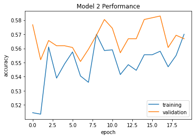
We can see that this model stabilizes just at 55%. Compared to the other model, this one doesn’t perform significantly better; if anything, it may have done slightly worse. However, we can see in the following plot that the accuracy and validation accuracy are much closer together than they were in the first model. Thus, we can conclude that this addition of rotations and flips reduced the issue of overfitting.
plt.plot(history.history["accuracy"], label = "training")
plt.plot(history.history["val_accuracy"], label = "validation")
plt.gca().set(xlabel = "epoch", ylabel = "accuracy", title="Model 2 Performance")
plt.legend()
Third Model
One thing that can be changed to improve performance is by transforming the given RGB values for each index to have a value between -1 and 1, or between 0 and 1. The following code block will transform our data so that it is optimized in this sense.
i = tf.keras.Input(shape=(160, 160, 3))
x = tf.keras.applications.mobilenet_v2.preprocess_input(i)
preprocessor = tf.keras.Model(inputs = [i], outputs = [x])
We will now incorporate this layer into our third model and see how it performs now.
model3 = models.Sequential([
    preprocessor,
    layers.RandomFlip(),
    tf.keras.layers.RandomRotation(0.2),
    layers.Conv2D(32, (3, 3), activation='relu', input_shape=(160,160, 3)),
    layers.MaxPooling2D((2, 2)),
    layers.Conv2D(32, (3, 3), activation='relu'),
    layers.MaxPooling2D((2, 2)),
    #layers.Conv2D(64, (3, 3), activation='relu'),
    layers.Dropout(0.2),
    layers.Flatten(),
    #layers.Dense(64, activation='relu'),
    layers.Dense(2) # number of classes
])
We will now train our new model and see how well it performs.
model3.compile(optimizer='adam',
              loss=tf.keras.losses.SparseCategoricalCrossentropy(from_logits=True),
              metrics=['accuracy'])

history = model3.fit(train_dataset,
                     epochs=20,
                     validation_data=validation_dataset)
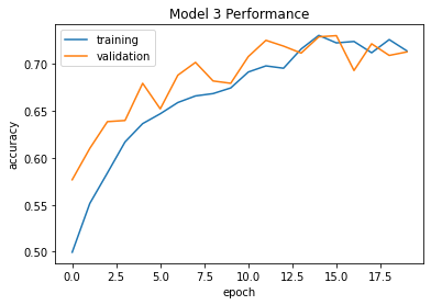
We can see that this model stabilizes between 70% and 72% for its validation accuracy. This model is significantly better than the first model we created. It also has a very close training accuracy, meaning we did not overfit our data.
plt.plot(history.history["accuracy"], label = "training")
plt.plot(history.history["val_accuracy"], label = "validation")
plt.gca().set(xlabel = "epoch", ylabel = "accuracy", title="Model 3 Performance")
plt.legend()
Fourth Model
For our last model, we will actually incorporate a model created by others that will help classify the images. To do this, we will first need to download MobileNetV2 and create it as a layer that we will use in our model.
IMG_SHAPE = IMG_SIZE + (3,)
base_model = tf.keras.applications.MobileNetV2(input_shape=IMG_SHAPE,
                                               include_top=False,
                                               weights='imagenet')
base_model.trainable = False

i = tf.keras.Input(shape=IMG_SHAPE)
x = base_model(i, training = False)
base_model_layer = tf.keras.Model(inputs = [i], outputs = [x])
Finally, lets create our last model.
model4 = models.Sequential([
    preprocessor,
    layers.RandomFlip(),
    tf.keras.layers.RandomRotation(0.2),
    base_model_layer,
    #layers.Conv2D(32, (3, 3), activation='relu', input_shape=(160,160, 3)),
    #layers.MaxPooling2D((2, 2)),
    #layers.Conv2D(32, (3, 3), activation='relu'),
    #layers.MaxPooling2D((2, 2)),
    #layers.Dropout(0.2),
    layers.Flatten(),
    layers.Dense(2) # number of classes
])
And now we will train this final model.
model4.compile(optimizer='adam',
              loss=tf.keras.losses.SparseCategoricalCrossentropy(from_logits=True),
              metrics=['accuracy'])

history = model4.fit(train_dataset,
                     epochs=20,
                     validation_data=validation_dataset)
We can see just how complex this model is by showing the summary.
model4.summary()
Model: "sequential_11"
_________________________________________________________________
 Layer (type)                Output Shape              Param #
=================================================================
 model (Functional)          (None, 160, 160, 3)       0

 random_flip_15 (RandomFlip)  (None, 160, 160, 3)      0

 random_rotation_11 (RandomR  (None, 160, 160, 3)      0
 otation)

 model_1 (Functional)        (None, 5, 5, 1280)        2257984

 flatten_10 (Flatten)        (None, 32000)             0

 dense_11 (Dense)            (None, 2)                 64002

=================================================================
Total params: 2,321,986
Trainable params: 64,002
Non-trainable params: 2,257,984
_________________________________________________________________
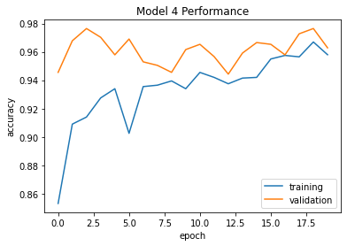
This model has a whole lot more paramters! However, only a small subset of them are trainable, with around 64,000 of them being trainable. We can also see that the model performs at about 95% to 97% validation accuracy. This models is clearly far superior than the other three! The training accuracy is also very close to the validation accuracy, so we do not suspect overfitting to occur.
plt.plot(history.history["accuracy"], label = "training")
plt.plot(history.history["val_accuracy"], label = "validation")
plt.gca().set(xlabel = "epoch", ylabel = "accuracy", title="Model 4 Performance")
plt.legend()
Final Testing
We will now see how the fourth and strongest model is at doing the classification on our test data.
y_pred = model4.predict(test_dataset)
labels_pred = y_pred.argmax(axis = 1)
loss, accuracy = model4.evaluate(test_dataset)
print("Test Accuracy :", accuracy)
6/6 [==============================] - 1s 59ms/step - loss: 0.4976 - accuracy: 0.9531
Test Accuracy : 0.953125
Just as we got on our validation set, this model had about a 95% to 96% accuracy rate. That’s pretty great at classifying dogs and cats!